Fine-tuning LLMs
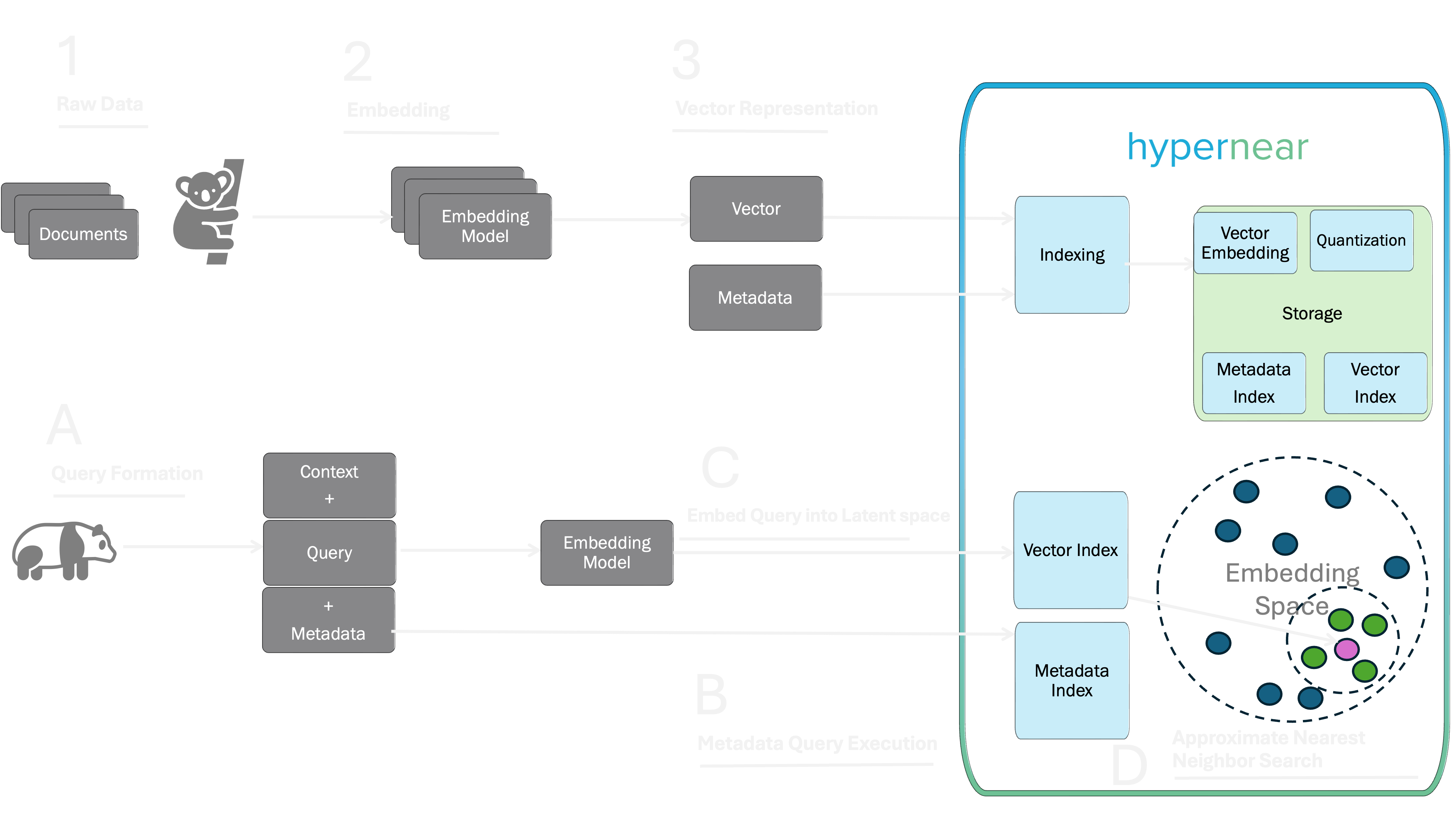
Vector databases index data based on data vectors or vector embeddings. Vector embeddings capture the meaning and context of data. High dimension vectors or scale 10^2, 10^3 or even higher capture more information, but they are harder to work with. We use these vectors to compute the distance between vectors, which can be used to indicate similarity between them.

When we run a query, we convert the given query into what we call 'query vector'. We now use a distance metric, a search algorithm and this query vector to retrieve a list of vectors that are closest to the given vector of your query,. Consider a massive multi dimensional dataset of vectors and a new query vector Q. We find the top k dataset vectors which are the most similar to Q. Let's first see how we measure a distance between two vectors, closer the vectors higher will be similarity score between them.
Distance Metrics
There are many different distance metrics used in KNN algorithm, we do support all major and promising distance metrics:
Cosine Distance
Considers the angle between two vectors to determine their similarity, considers both the direction and magnitude of vectors and disregards the length of the vectors.
Dot Product Distance
Considers only magnitudes of the vectors matter, and the direction becomes less relevant
Chebyshev Distance
Calculates the sum of absolute differences of their 2-dimensional coordinates.
Manhattan Distance
Calculates the distance by summing the absolute differences along each dimension. They are preferred for high dimensionality data.
Euclidean Distance
Calculates the cartesian distance between the two points which are in the plane/hyperplane
Hamming Distance
Computated as how many changes are needed to convert one vector to the other
As a rule of thumb, it is best to use the distance metric that matches the model that you're using. Choice of distance metric depends on your data, model, and application. Such similarity searches are used by systems such as voice recognition, image / video retrieval, and recommendation systems; more recently it has been brought to the forefront of generative AI as one of the main drivers to improve performance through Retrieval-Augmented Generation (RAG).
Vector Indexing available in hypernear
Instead of comparing vectors one by one, we use Approximate Nearest Neighbor (ANN) algorithms. ANN algorithms may not return the true k nearest vectors, but they are very efficient. ANN algorithms maintain balance between the performance and search results on very large-scale datasets. Hypernear expose customisation parameters to configure how ANN algorithm should behave. This lets you find the right balance between the recall tradeoff results, latency, throughput and import time.
Data vectors are stored as indexes that allow efficient lookup for vectors. The embedding models used typically stores vectors with a dimensionality of the order of 10^2 or 10^3 or even higher. ANN algorithms techniques thus attempts to capture the actual complexity of the data as efficiently as possible in time and space.
Flat Index
Flat indexing is an index strategy where we simply store each vector as is, with no modifications. It is easy, accurate but slow. Flat indexing is the right choice when perfect accuracy is required and speed is not a consideration. For small datasets, flat indexing may also be a good choice as the search speed can still be reasonable.
LSH Indexing
The index is built using a hashing function. When performing a query, the hash function of the query is computed and mapped values from the hash table are taken. Each of these mapped values contains its own set of potential candidates which then are further checked on the query condition to be the neighbours.
Inverted File indexing
also called postings list indexing, implemented using posting list data structure is a index storing a mapping from content to its locations in the latent space. We partition the latent space using centroids.
HNSW
Hierarchical Navigable Small World (HNSW) is a state of the art, proximity graph algorithm and index type, it works on multi-layered graphs by marrying the swift traversal of skip lists with NSW’s interconnectivity.
HNSW indexes enable very fast queries, but rebuilding the index can be resource intensive. At the build time, the HNSW algorithm creates a series of layers. At query time, it uses these layers to build a list of approximate nearest neighbors (ANN) quickly and efficiently. Different layers have different number of data vector objects stored, the lowest layer often refered as layer 0 stores each data vector object and they are well connected to each other. As we move upwards, we have fewer data vector object and hence fewer connections.
HNSW enables very fast queries with this style of hierarchical layers of graphs, by entering from top layer starting closest matching points.
HNSW is very fast, memory efficient, approach to similarity search. We expose important configuring construction and query search parameters like the size of the dynamic list for the nearest neighbors, the number of nearest neighbors to be returned as the result, the number of bi-directional links created for every new element during construction which help you to fine tune the indexing.
Try hypernear that has all of the benefits of best of indexing mechanisms
and configurability of choosing distance metric based on your data, model and application.

